Neutrinos

Introduction

The name neutrino was coined to describe a then hypothetical particle suggested by Wolfgang Pauli in the 1930's. Pauli's idea was that of a neutral, weakly interacting particle having a very small mass. He proposed this particle could be used to explain the spectrum of electrons emitted by $\beta$ -decays of atomic nuclei, which was of considerable controversy at the time. The observed spectrum of these electrons is continuous, which is incompatible with the two-body decay description successfully used to describe discrete spectral lines in $\alpha$- and $\gamma$- decay of atomic nuclei. As Pauli observed, by describing $\beta$-decay as a three-body decay instead, releasing both an electron and his proposed particle, one can explain the continuous $\beta$-decay spectrum. Soon after discovery of the neutron, Enrico Fermi used Pauli's light neutral particle as an essential ingredient in his successful theory of $\beta$-decay, giving the neutrino it's name as a play on words of little neutron in Italian.

It was not until some 20 years later that the discovery of the neutrino was realised. It was eventually understood that neutrinos came in three distinct flavours $\left (\nu_e,\nu_\mu,\nu_\tau\right )$ along with their associated antiparticles $\left (\bar\nu_e,\bar\nu_\mu,\bar\nu_\tau\right)$.

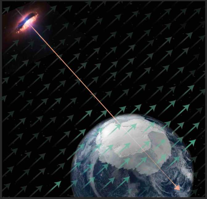
I am particularly interested in the study of astrophysical neutrinos which are ones that are very-high-energy and come from astrophysical origins such as Active Galactic Nuclei. Neutrinos are electrically neutral, so are not perturbed by interstellar magnetic fields, and they also have a small enough interaction cross-section to escape from dense regions. This makes them ideal messengers to help identify the origins and accelerations mechanisms of ultra-high-energy cosmic rays, a long standing puzzle in astrophysics.

Research with IceCube

The IceCube neutrino observatory is a cubic kilometre photomultiplier array embedded in the extremely thick and clear glacial ice located near the geographic South Pole in Antarctica. The IceCube array is made up of 5160 purpose built Digital Optical Modules (DOMs) which are deployed on 86 cables between 1450 and 2450 m below the ground. The interaction of a neutrino releases a burst of light in the detector, which is detected by this array of DOMs. The timing and intensity of these photons form the raw data set at IceCube. This data is analysed so that we can learn more about the properties of neutrinos. You can checkout some cool animations of how an event looks like in IceCube on this website.

Search for Quantum Gravity

The Standard Model (SM) of particle physics and Einstein’s theory of general relativity predicts known phenomena in Nature from small to large scales, such as existence of Higgs boson and gravitational waves. However, we yet do not have a single theory to describe both, a dream theory of all physicists, known as quantum gravity (QG). QG describes the unification of all particles, forces, and space-time. QG effects are expected to appear at the ultra-high-energy scale called the Planck energy, $E_P\equiv1.22\times10^{19}$ GeV. However, such a high-energy world would exist only in the moment of the Big Bang. On the other hand, it is speculated that the effects of QG may exist in our low-energy world, but are suppressed as the inverse of the Planck energy ($1/E_P$, $1/E_P^2$ , $1/E_P^3$, etc.). This can be due, for example, by new field, remnant of the Big Bang, saturating vacuum and causing an anomalous space-time effect.

I first worked on searching for such new physics using atmopherically produced neutrinos. At the time, it provided the best attainable limits in the neutrino sector and the best limits on certain parameters across all fields of physics. This work was published in Nature Physics. I then went on to work on searching for new physics using astrophysical neutrino flavour information, where for the first time our limits reached the signal region of QG-motivated physics: the QG frontier.

Bayesian inference

Introduction

Data is stochastic in nature, so an experimenter uses statistical methods on a data sample $\textbf{x}$ to make inferences about unknown parameters $\mathbf{\theta}$ of a probabilistic model of the data $\left(\textbf{x}\middle|\mathbf{\theta}\right)$. The likelihood principle describes a function of the parameters $\mathbf{\theta}$, determined by the observed sample, that contains all the information about $\mathbf{\theta}$ that is available from the sample. Given $\textbf{x}$ is observed and is distributed according to a joint probability distribution function (PDF), $\left(\textbf{x}\middle|\mathbf{\theta}\right)$, the function of $\mathbf{\theta}$ which is defined by

$$ L\left(\mathbf{\theta}\middle|\textbf{x}\right)\equiv f\left(\textbf{x}\middle|\mathbf{\theta}\right) $$

is called the likelihood function. In a Bayesian approach, $\theta$ is considered to be a quantity whose variation can be described by a probability distribution (called the prior distribution), which is subjective based on the experimenter's belief. when an experiment is performed it updates the prior distribution with new information. The updated prior is called the posterior distribution and is computed through the use of Bayes' Theorem

$$ \pi\left(\mathbf{\theta}\middle|\textbf{x}\right)=\frac{f\left(\textbf{x}\middle|\mathbf{ \theta}\right)\pi\left(\mathbf{\theta}\right)}{m\left(\textbf{x}\right)} $$

where $\pi\left(\mathbf{\theta}\middle|\textbf{x}\right)$ is the posterior distribution, $\left(\textbf{x}\middle|\mathbf{\theta}\right)\equiv L\left(\mathbf{\theta}\middle|\textbf{x}\right)$ is the likelihood, $\pi\left(\mathbf{\theta}\right)$ is the prior distribution and $\left(\textbf{x}\right)$ is the marginal distribution,

$$ m\left(\textbf{x}\right)=\int f\left(\textbf{x}\middle|\mathbf{\theta}\right)\pi\left( \mathbf{\theta}\right)\text{d}\mathbf{\theta} $$

Markov Chain Monte Carlo

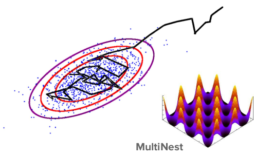
The goal of a Bayesian inference is to maintain the full posterior probability distribution. The models in question may contain a large number of parameters and so such a large dimensionality makes analytical evaluations and integrations of the posterior distribution unfeasible. Instead the posterior distribution can be approximated using Markov Chain Monte Carlo (MCMC) sampling algorithms. As the name suggests these are based on Markov chains which describe a sequence of random variables $\Theta_0,\Theta_1,\dots$ that can be thought of as evolving over time, with probability of transition depending on the immediate past variable, $\left(\Theta_{k+1}\in A\middle|\theta_0,\theta_1,\dots,\theta_k\right)= P\left(\Theta_{k+1}\in A\middle|\theta_k\right)$.

In an MCMC algorithm, Markov chains are generated by a simulation of walkers which randomly walk the parameter space according to an algorithm such that the distribution of the chains asymptotically reaches a target density $\left(\theta\right)$ that is unique and stationary (i.e. no longer evolving). This technique is particularly useful as the chains generated for the posterior distribution can automatically provide the chains of any marginalised distribution, e.g. a marginalisation over any or all of the nuisance parameters.

Anarchic Sampling

As with any Bayesian based inference, the prior distribution used for a given parameter needs to be chosen carefully. In my analysis, a further technology needed to be introduced in order to ensure the prior distribution is not biasing any drawn inferences. Since we were using MCMC techniques, the space in we sample in needs to be chosen carefully. A nice way to see this is by using the example of randomly choosing points on a unit sphere. In polar coordinates, if we sample uniformally in $\theta\in[0,2\pi)$ (polar) and $\phi\in[0,\pi)$ (azimuthal) then we find that the points we have picked bunch up around the poles. Checkout the animation below to see a visualisation of this. To sample correctly, without introducing any artificial biases, we must sample in the integration invariant area element

$$ \text{d}\Omega=\sin\theta\text{ d}\theta\text{ d}\phi= -\text{d}\left(\cos\theta\right)\text{ d}\phi $$

i.e. we must sample uniformally in $\cos\theta\in[-1,1]$ and $\phi\in[0,\pi)$.

GolemFlavor Bayesian Inference Python package

The code which I wrote for the IceCube astrophyical flavour analysis is available on GitHub and is packaged as GolemFlavor.